Page 81 - 068

67

th
ˆ
  4 Moment .
 
3  2 2
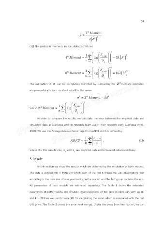
(12) The particular moments are calculated as follows

n   S   4
1 t  t 2
4 Moment  th   log  i   3    
2

n i 1     S t i    
n   S   6
1 t  t 3

6 Moment  th   log  i    15    .
2
n i 1     S t i    
The estimation of  can be completely identified by subtracting the 2 moment estimated
nd
nonparametrically from constant volatility, this mean

ˆ
  2 2 Moment  nd 
2
n   S   2
1 t  t
nd
where 2 Moment    log  i   .
n i 1     S t i    
In order to compare the results, we calculate the error between the empirical data and

simulated data as Maekawa and his research team use in their research work (Maekawa et al.,

2008). We use the Average Relative Percentage Error (ARPE) which is defined by

1 M x  s
ARPE   i i , (13)
M i 1 x i

where M is the sample size, x and s are empirical data and simulated data respectively.
i i
5 Result

In this section we show the results which are obtained by the simulation of both models.

The data is divided into 6 groups in which each of the first 5 groups has 250 observations that

according to the data size of one year trading in the market and the last group contains the rest.

All parameters of both models are estimated separately. The Table 1 shows the estimated

parameters of both models. We simulate 2000 trajectories of the price in each part with Eq. (6)
and Eq. (7) then we use formula (13) for calculating the errors which is compared with the real

USS price. The Table 2 shows the errors that we get. Under the same Brownian motion, we can