Page 83 - 068

69

where x is the Gaussian random number and a , b are the typical value of volatility in the real
market which are 15 % and 60 % respectively. Then, we again simulate as the previous one. The
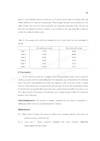
Table 3 shows the new errors that we get after we change the estimation of ˆ  . We can see
d
that even we change the value of volatility to be according to the real market the continuous

model still provide the better errors.

Table 3. The average errors which are obtained by both models after the new estimation of
ˆ  (%)
d
The continuous model The model with jumps
Data 1 13.92 24.25

Data 2 42.04 68.53
Data 3 21.82 40.42
Data 4 27.87 32.17
Data 5 21.63 31.62

Data 6 24.18 51.31

6 Conclusion

In this study we provide the simulation of the Thailand natural rubber price by using the
continuous model and the model with jumps. The parameters are estimated from the historical

price. The results show that the errors which are obtained by the continuous model is smaller
than the model with jumps compare with the real USS price. Since the first spotted large change
in the USS price we expected the model with jumps would provide the better error but it is not.

This maybe because of the jumps in the USS price are not large enough to affect the continuous
behavior of this USS price.

Acknowledgements This research is partially supported by the Centre of Excellence in
Mathematics, the Commission on Higher Education, Thailand.

References

[1] F. Black and M. Scholes, The pricing of options and corporate liabilities, The journal of

political economy, (1973), 637-654.

[2] R. Cont and P. Tankov, Financial Modelling with Jump Processes. 133(2004),

Chapman&Hall/CRC Boca Raton.