Page 79 - 068

65

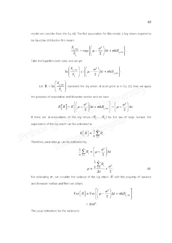
model we consider from the Eq. (6). The first assumption for this model is log return required to
be Gaussian distribution this means

S     2  
t  t  exp     t    B  .
 
i
S   2  t  t 
i
t i   
Take the logarithm both sides and we get
 S      2  
ln  t  t       t    B  .
 
i
 S    2  t  t
i
 t i     
 S 
Let R  ln  t  t  represent the log return of asset price as in Eq. (1), then we apply
i
 S 
 t i 
the property of expectation and Brownian motion and we have

   2     2
E R   E       t    B         t  .
 

 2   t  t    2 
i
If there are n observations of the log return (R ,...,R ) by the law of large number the
1 n
expectation of the log return can be estimated as

1
n
E R   n  R .


i
Therefore, parameter  can be estimated by i 1
1 n    2
R      t 
n i 1 i   2  

n
1  R
n i  2
  i 1  . (8)
t  2

For estimating  , we consider the variance of the log return R with the property of variance
and Brownian motion and then we obtain

   2 
Var R    Var     t    B 
 
  2    t  t  
i
  t .
2
The usual estimation for the variance is