Page 44 - 048

26

2
2
2
Y=  0 +  1X 1 +  2X 2 +  3X 3 +  11X 1 +  12X 1X 2 +  13X 1X 3 +  22X 2 +  23X 2X 3 +  X (3.1)
3
33

Where Y is the predicted response; X 1, X 2 and X 3 are the parameters;  0 is the offset
term;  1,  2 and  3 are the linear coefficients;  11,  22 and  33 are the squared coefficients; and
 12,  13 and  23 are the interaction coefficients. The response variable was fitted using a
predictive polynomial quadratic equation (Eq. (3.1)) in order to correlate the response variable to
the independent variables (Lay, 2000). Table 3.2 and Table 3.3 illustrate the code values of the
variables, the conditions of each run and the corresponding results.

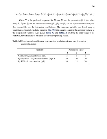
Table 3.2 Experimental variables and concentration levels investigated by using central
composite design.

Variable Parameter value
-1 0 1
X 1: NaHCO 3 concentrations (g/L) 3 6 9
X 2: Na 2HPO 4.12H 2O concentrations (mg/L) 0 10 20
X 3: EFB ash concentration (g/L) 0 15 30